
[Paper] Convection-permitting scales break climate invariance in machine-learned precipitation downscaling
Preprint · September 2026
Convection-permitting scales break climate invariance in machine-learned precipitation downscaling
Climate models compute rain on grids 25 to 100 km wide, too coarse for the downpours that flood a neighborhood. Running a weather model fine enough to resolve individual thunderstorms (about 3 km) over decades is far too expensive, so a common shortcut is machine-learned downscaling: train a neural network to turn coarse rain fields into fine ones. Networks are trained on today’s climate and then applied to the future, which quietly assumes that the relation between coarse and fine rain does not change as the climate warms. This assumption is known as climate invariance (Beucler et al., 2024). We tested it over Puerto Rico and found no detectable change at coarse resolution, but a significant break at the step where thunderstorms start to be resolved.
1 One network for each step, 48 → 25 → 12 → 3 km
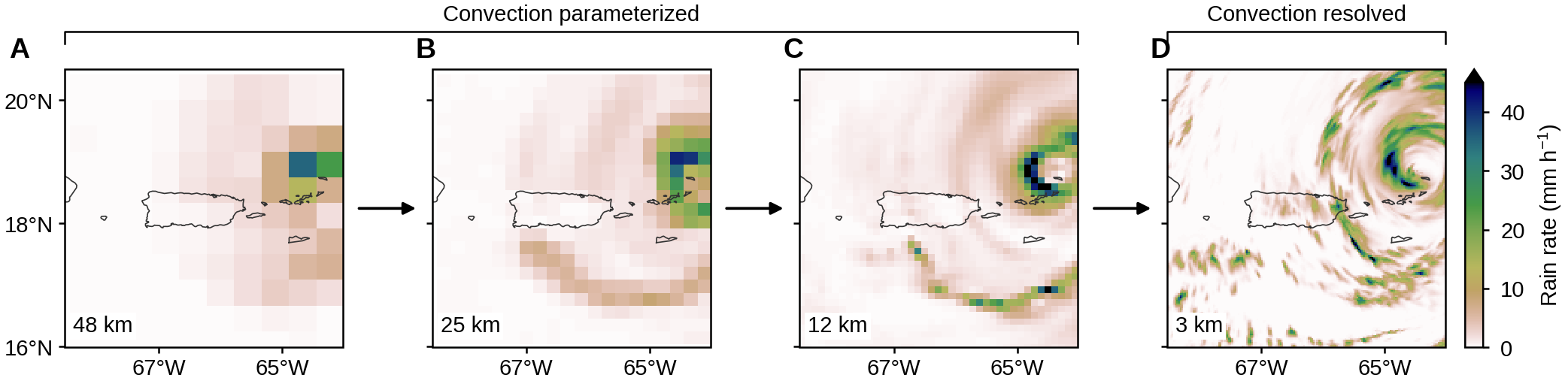
Erin selected extreme-rain days from an ensemble of ten climate-model runs (Dougherty et al., 2026): 78 days in 2001–2021 and 77 days in 2041–2061 under a high-emission scenario (RCP8.5). Each day was simulated for 36 hours with the weather model MPAS at 48, 25, 12 and 3 km, and a separate network, a generative adversarial network (GAN) that learns to draw realistic detail, was trained for each step (Fig. 1). Only the 3-km grid resolves thunderstorms (convection), which is why such grids are called convection-permitting; the coarser grids represent thunderstorms with a simplified rule, a parameterization.
2 Networks trained in two climates, given the same input
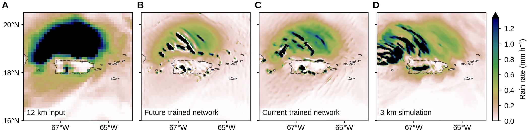
Every step was trained twice, once on current-climate days and once on near-future days. To see whether the learned relation depends on climate, we gave both versions the same future input and compared their output with the simulation on the finer grid (Fig. 2). By eye the two outputs look much alike; the difference shows up in the statistics of many hours (Fig. 3).
3 No detectable climate dependence at the coarse steps; a significant one at 12 → 3 km
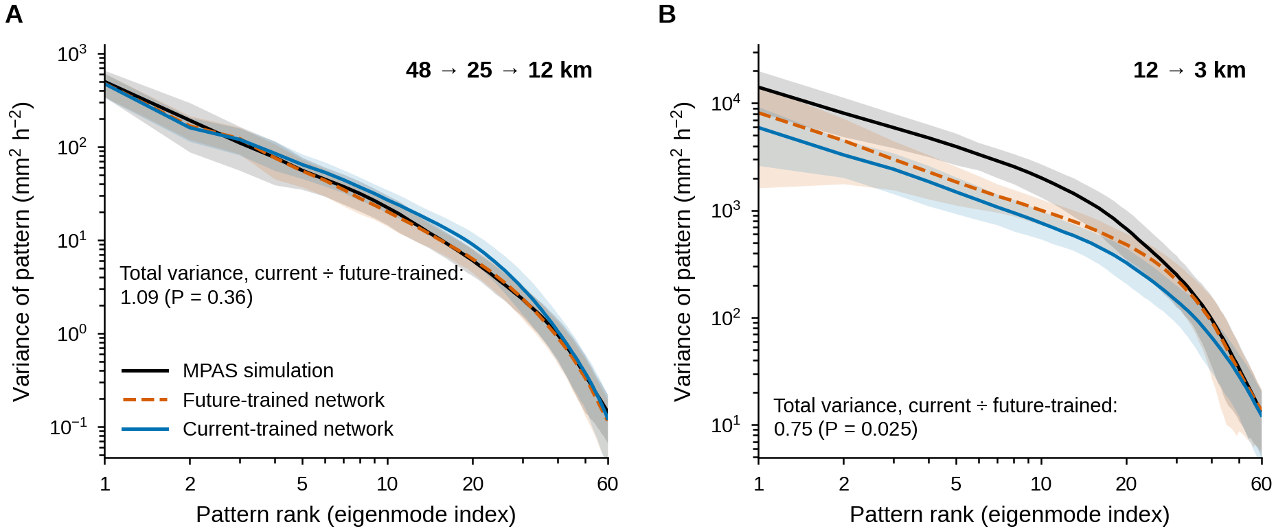
We took 468 hours (36 per simulated day) from 13 future days held out of training, split the rain into spatial patterns ranked by how much variability they carry, and plotted the variance of each pattern, largest first (an eigenspectrum, as in principal component analysis; Fig. 3). For the coarse steps the two networks agree: the ratio of their total variance is 1.09, with no detectable difference from 1 (P = 0.36). At 12 → 3 km, the future-trained network recovers 56% of the simulated variance (downscaling networks tend to be too smooth), and the current-trained network only 42%, a quarter less (ratio 0.75, P = 0.025). Even with the correct future input, the network trained on today’s storms underestimates the variability of future storms more than the network trained on future storms does.
4 A likely reason: warming adds energy at scales a 12-km grid cannot carry
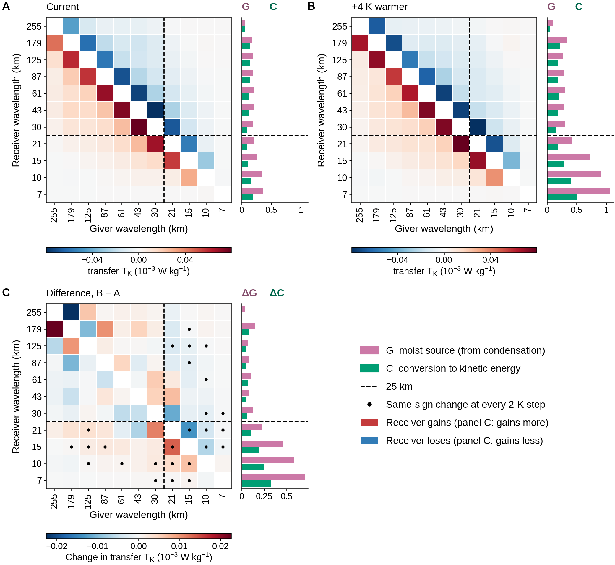
To find the physical reason we simulated an idealized squall line, a line of thunderstorms in a simplified setting (Weisman and Klemp, 1982), with the surface warmed by 0 to 8 K in 2-K steps, and split its energy budget by wavelength (Augier and Lindborg, 2013; Fig. 4). Condensation heating (G) is the energy input, part of it is converted into motion (C), and the motion exchanges kinetic energy between scales. Warming does not make the conversion more efficient (the fraction of G turned into motion is 0.57 today and 0.51 at +4 K); it supplies more heating.
With 4 K of warming, G grows by 168% at wavelengths below 25 km but by 52% above, so about 75% of the extra input lands at the small scales. Every exchange between scales that changes steadily with warming also involves those small scales. A 12-km grid cannot represent waves shorter than 24 km, twice its spacing, and 25 km is the nearest band edge. This points to the climate signal entering through scales absent from the coarse input, which a network can only supply from what it learned in training.
In short, the coarse steps of a downscaling chain could be reused in a warmer climate in our test, but the step into thunderstorm-resolving scales needs retraining or explicit information about the climate. Because the error depends on scale, a single correction factor, such as scaling rain by about 7% per degree of warming (roughly how much more water vapor warmer air can hold), is unlikely to fix it. The preprint also tests a simpler statistical method, the ensemble-conditional Gaussian process, with the same conclusion.
Thanks to my coauthors: Anamitra Saha (IIT Hyderabad), who developed the downscaling networks; Erin Dougherty (NSF NCAR), who selected the extreme days and ran the MPAS simulations; and Sai Ravela (MIT).
Preprint: X. Yan, A. Saha, E. M. Dougherty, S. Ravela, “Convection-permitting scales break climate invariance in machine-learned precipitation downscaling,” Research Square (2026), doi:10.21203/rs.3.rs-10899014/v1.