
[Paper] Ensemble-Conditional Gaussian Processes (Ens-CGP): Representation, Geometry, and Inference
Preprint · February 2026
Ensemble-Conditional Gaussian Processes (Ens-CGP): Representation, Geometry, and Inference
Much of geoscience comes down to estimating a whole field, such as temperature or rain on a grid, from a few noisy measurements plus prior knowledge, which often comes from an ensemble of model runs. The task goes by several names, taught in different courses: kriging, regularized least squares, kernel ridge regression and the Kalman filter. This preprint lays out why, under Gaussian assumptions, they give the same estimate, and what changes when the prior comes from an ensemble. Here are the four main points.
1 Four methods, one formula
Take a prior, what is believed before the data, for the field \(f\) (a vector of \(n\) values on a grid), with mean \(m\) and covariance \(K\) (how values at different places vary together), and noisy linear measurements \(y = Hf + \varepsilon\), where \(H\) picks out what was observed and the noise \(\varepsilon\) has covariance \(R\). The field given the data, the posterior, is Gaussian with
\[ m_{\rm post} = m + G\,(y - Hm), \qquad K_{\rm post} = K - GHK, \qquad G = KH^{\mathsf T}\,(HKH^{\mathsf T} + R)^{-1}. \]The gain \(G\) sets how strongly the misfit \(y - Hm\) corrects the prior. Simple kriging, the geostatistics method for interpolating a field from scattered measurements with a known mean, computes exactly this. Regularized least squares, which fits the data while penalizing fields the prior finds unlikely (misfit weighted by \(R^{-1}\), penalty by \(K^{-1}\)), gives the same mean. Kernel ridge regression, which treats \(K\) as a similarity between points, gives it too when its ridge weight equals the noise variance (the same at every observation) and the prior mean is subtracted first. And the update step of the Kalman filter, used throughout data assimilation (combining model forecasts with observations), is the same formula applied each time new observations arrive. The preprint calls the underlying object a conditional Gaussian process (CGP): a Gaussian distribution over whole fields, conditioned on the data.
2 Any square root of the covariance gives the same answer
Write \(K = AA^{\mathsf T}\). The columns of \(A\) can be eigenvectors of \(K\) scaled by the square roots of their eigenvalues, or, when \(K\) is an ensemble covariance, the members minus their mean divided by \(\sqrt{E-1}\) for \(E\) members; any matrix \(B\) with \(BB^{\mathsf T} = K\) gives the same posterior. When \(K\) has low rank \(r\), as an ensemble covariance does, the calculation can use a thin factor with \(n\) rows and only \(r\) columns, without ever forming the full \(n\times n\) matrix.
3 With an ensemble as the prior, the data can only move the field in directions the ensemble spans
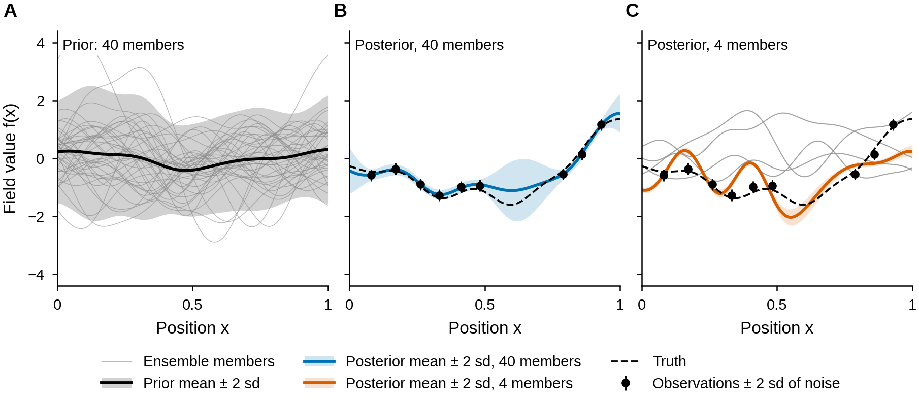
Ens-CGP (the ensemble-conditional Gaussian process) uses the ensemble mean as \(m\) and the ensemble’s sample covariance as \(K\), with the columns of \(A\) being the \(E\) members minus their mean, divided by \(\sqrt{E-1}\), and then conditions exactly. Every correction is a combination of those columns, so the data can only change the field in directions the ensemble already spans (a combination can still go outside the range of the individual members). Fig. 1 shows a one-dimensional test made for this page: a smooth field on the interval from 0 to 1, observed at 9 points with noise of standard deviation 0.1. With 40 members, the posterior mean has a root-mean-square error of 0.20 across the interval and its ±2-standard-deviation band contains the truth at 100% of points. With 4 members there are only 3 directions (subtracting the mean costs one), and the error rises to 0.58. Because the uncertainty also lives only in those directions, which the 9 observations pin down, the band is narrow and covers the truth at only 21% of points. The ensemble Kalman filter (Evensen, Ocean Dynamics, 2003), which gives each member its own copy of the data perturbed with random noise, is a randomized way of computing Ens-CGP: its mean matches up to that randomness.
4 Reusing the same data is not new information
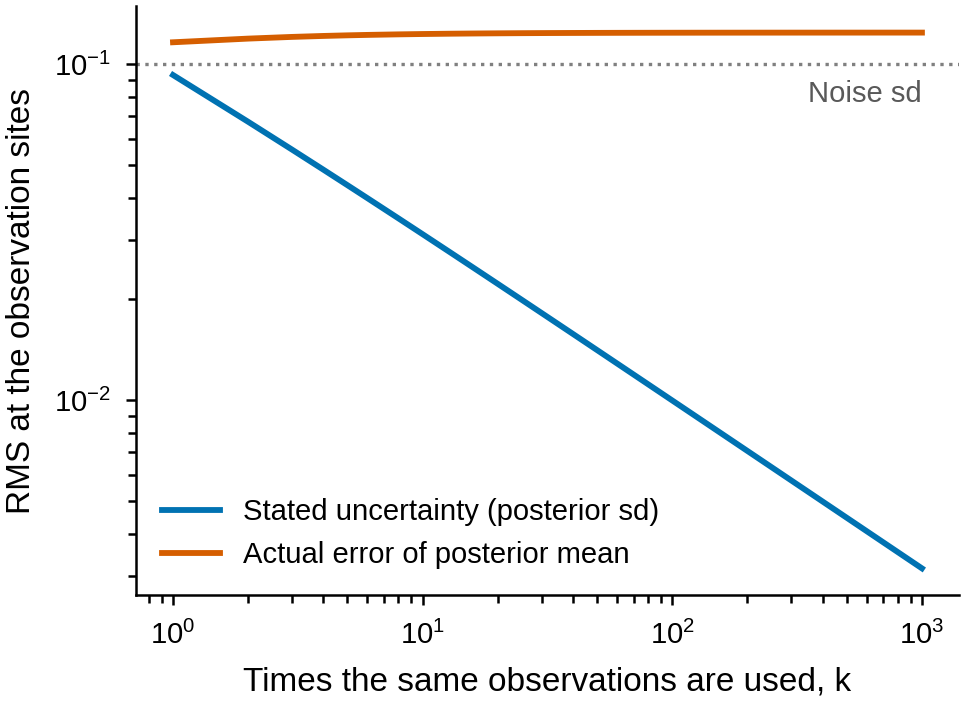
Some iterative ensemble schemes, which refine an estimate step by step, feed the same observations back in at every iteration. That is equivalent to treating one measurement as \(k\) independent ones, i.e. replacing the noise covariance \(R\) by \(R/k\). The stated uncertainty then keeps shrinking while the error does not (Fig. 2): after 1000 uses, our example claims an uncertainty of 0.0032 at the observation sites, while its actual error there is 0.124, 39 times larger. Such schemes are better viewed as optimization that needs a stopping rule; they remain correct probability (Bayesian) updates only if each pass brings new data, or if the noise is inflated so that all passes together add up to a single update.
Ens-CGP underlies several projects in the group: in precipitation downscaling it estimates fine rain from coarse rain; in magnetotelluric inversion, which maps underground electrical resistivity from surface measurements, it provides the first guess that a neural network then corrects (Kim, Ravela and Evans, 2026); and it is a natural first guess for the boosting ladder, a sequence of learned corrections.
Preprint: S. Ravela, J. D. Kim, K. Gee, X. Yan, S. Mercier, L. Albarghouty, A. Saha, “Ensemble-Conditional Gaussian Processes (Ens-CGP): Representation, Geometry, and Inference,” arXiv:2602.13871 (2026).