
Correcting a coarse forecast rung by rung: stable boosting in time
Research article · Estimation theory and machine learning
Correcting a coarse forecast rung by rung: stable boosting in time
Department of Earth, Atmospheric and Planetary Sciences, Massachusetts Institute of Technology, Cambridge, MA, USA.
A coarse weather model resolves large-scale flow but not the detail that a fine model adds. We estimate the fine field as a ladder of corrections: a linear first guess, then a sequence of small models, the rungs, each fitted to what the rungs before it still get wrong. Unlike classical boosting, a machine-learning method that adds simple models one after another, every rung carries part of its previous hour's estimate into the next hour, because the error of a forecast persists in time. On a synthetic one-dimensional problem we examine two conditions specific to time: each rung is trained exactly as it is used, running forward hour by hour on its own estimates rather than on the true past error, which for the first rung gives a small but consistent improvement; and the fraction carried from one hour to the next stays below 1, which by construction makes a mistake fade instead of grow. A third, classical condition is that the number of rungs is chosen on runs not used for fitting. On 60 test runs, never used for fitting or choices, the rungs lower the root-mean-square error (RMSE) at every one of the 73 hourly times (hours 0 to 72), from 0.664 to 0.367 with rungs 0 to 15 added at full size. When each correction is instead added at a fraction of its size (small steps), the validation error is nearly the same but the corrections keep shrinking, and the error settles at the size of the small-scale texture that the coarse input cannot predict. A final random rung, which draws that texture at random, reproduces how fast it changes from hour to hour, approximately.
Weather models are run on grids, and a fine grid costs far more than a coarse one. Downscaling estimates, from a coarse-grid forecast alone, the field that a fine-grid forecast would produce. Statistical first guesses are often linear. A conditional Gaussian mean, the best linear estimate of the fine field given the coarse one when both are treated as jointly Gaussian, maps the coarse field onto the fine grid; the mean of an ensemble-conditional Gaussian process, a method that treats the fields as random values whose correlations are estimated from an ensemble, here a large collection of past cases, is an example (1); it is context here, and nothing below depends on its details. What such a map misses is not random noise. Part of it depends on the past of the flow, such as a response that lags its cause by hours, and part is small-scale texture whose position no coarse input determines.
An error with memory calls for a model of the error that also has memory. Machine-learned corrections to imperfect models of dynamical systems include corrections with memory (2); recurrent neural networks, which carry a state from one time step to the next, can represent the time integration of continuous dynamics (3); and a learned correction on top of an ensemble-based first estimate has improved the recovery of Earth's electrical structure from surface measurements (4).
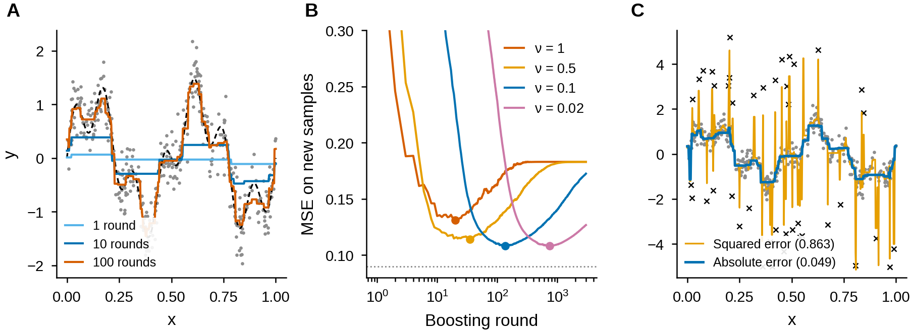
Gradient boosting (5), a machine-learning method that builds a predictor as a sum of many simple models, supplies the second ingredient: each simple model is fitted to what is still wrong, added with a fraction ν of its full size (the step size), and the sequence stops when the error on held-out data, data not used for fitting, stops improving. Successive correction is an old idea in the geosciences as well; scale-cascaded alignment, for instance, estimates how far features in one field must move to match another, one band of spatial scales at a time (6). Here we combine the two ideas in time. We ask whether the corrections shrink, what they converge to, and what keeps an error model with memory from amplifying its own mistakes.
A ladder of corrections
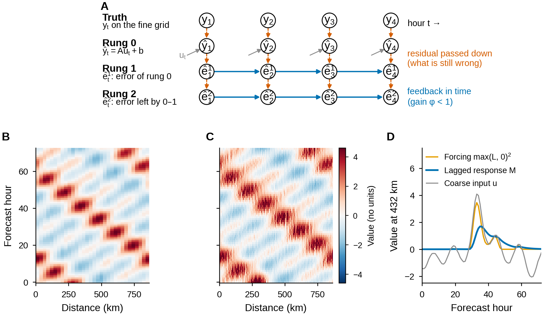
Let ut be the coarse input at hour t and yt the fine truth; a hat marks an estimate. Rung 0 is linear (Fig. 1A):
ŷ(0)t = A ut + b,
with a fitted matrix A and offset b. Rung n ≥ 1 estimates what rungs 0 to n − 1 leave, the residual yt − ŷ(n−1)t, with a recursion that carries its own previous estimate forward:
ê(n)t = φn ê(n)t−1 + (1 − φn) βn·zt, ŷ(n)t = ŷ(n−1)t + ν ê(n)t.
Here zt are features, quantities computed from the data: for rung 1, the coarse input near each point; for later rungs, fixed random curved functions of that input and of the current estimate ŷ(n−1)t (Materials and Methods). Rung 1 is therefore the error model of rung 0; βn are fitted weights, and φn, the feedback gain of rung n, is the fraction of the previous hour's estimate carried into the next; each rung has one gain. Because the fine truth is never available when the method is used, the recursion carries the model's own past estimate, never the true past error. For a fixed φn the recursion is an exponentially weighted average of recent features (a linear filter), êt = Σj≥0 (1 − φ) φj β·zt−j. Fitting it on its own rollout, that is, with the model run forward hour by hour on its own outputs exactly as in use, therefore reduces to a ridge regression (least squares with a small penalty on the size of the weights) on exponentially filtered features. Each φn is chosen by out-of-fold error: the training runs (the 72-hour realizations used for fitting; see the test problem below) are split into five groups, each group is predicted by a fit to the other four, and the error of these predictions decides among candidate values.
The feedback also bounds the error. A mistake δ made at one hour is still present as φhδ after h hours. With φ < 1 the accumulated effect of mistakes no larger than ε per hour stays below ε/(1 − φ); with a gain above 1 it grows without limit.
A test problem
The test problem is synthetic, and its field values are dimensionless. A line of 864 km, periodic so that its right end joins its left end, is seen by a coarse model in 32 cells of 27 km and by a fine model at 288 points of 3 km, hourly from hour 0 to hour 72 (Fig. 1, B and C). A run is one such 72-hour realization; there are 240 training runs used for fitting, 60 validation runs used for every choice, and 60 test runs scored once at the end. The fine truth is y = L + M + S: L is a set of large travelling waves, one to three wavelengths across the domain, that the coarse model also sees; M is a response that relaxes toward its forcing max(L, 0)2, the square of the positive part of the waves, with a memory of 6 hours, meaning that each hour keeps a fraction e−1/6 ≈ 0.85 of the previous hour's response; it starts equal to its forcing at hour 0 (in balance), which is why errors are lowest at hour 0 (Fig. 1D); and S is small-scale texture, finer than the coarse grid can represent, whose amplitude grows with the waves but whose position is random. The coarse model sees the waves, responds to the forcing at once and too weakly, and has a slowly varying error of its own. The simplest baseline is the coarse field linearly interpolated between the centers of the coarse cells. Errors are the root-mean-square error (RMSE), the square root of the mean squared difference from the truth, averaged over all points, hours and runs unless a figure shows them by hour. Results below say whether a number comes from the validation or the test runs, which differ slightly.
Results
A linear first guess leaves an error with memory
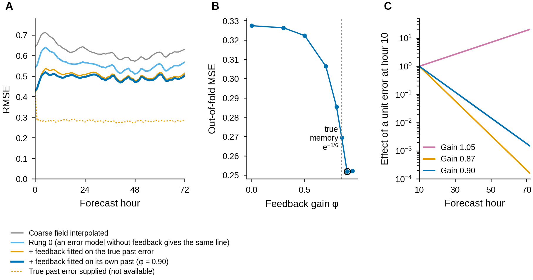
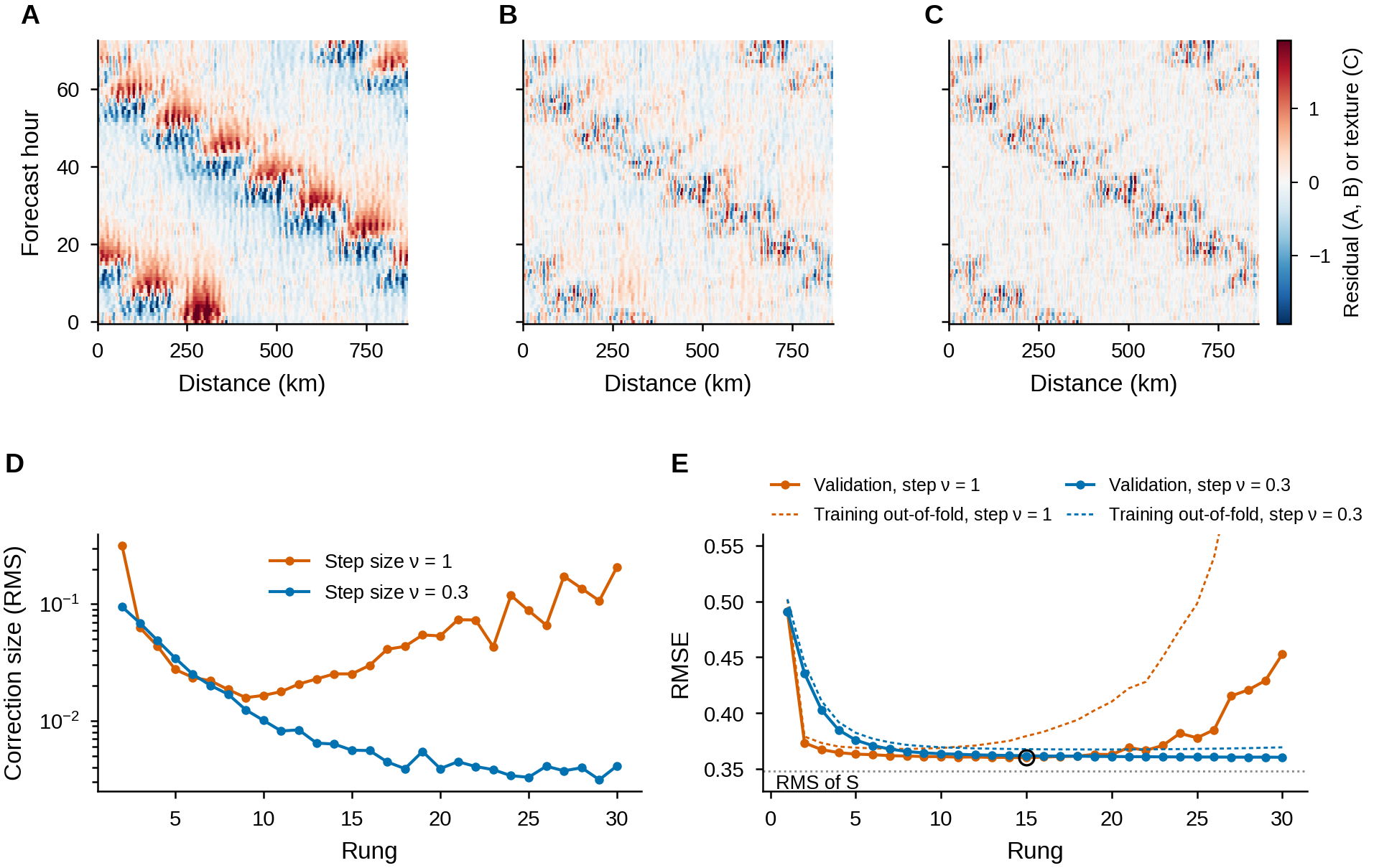
The linear first guess lowers the validation RMSE from 0.620 for the interpolated coarse field to 0.555 (Fig. 2A). What it leaves is structured: wide bands that follow the lagged response, plus fine-grained texture (Fig. 3A). A second linear model of the same input, without feedback, adds nothing (0.555).
Feedback must be trained the way it is used, and must fade
Adding feedback lowers the error to 0.491 when the error model is fitted on its own rollout, with a gain chosen by the data, φ1 = 0.90 (Fig. 2B), close to the true memory of the response, e−1/6 = 0.85. The same model fitted with the true past error in place of its own estimate, and then run on its own, ends up with a gain of 0.87 and scores 0.501 on the validation runs, about 2% worse. It is worse at 71 of the 73 hourly times; consecutive hours are strongly correlated, so this shows a consistent small difference, not 73 independent tests. Scored with the true past error, which is never available in use, it would appear to reach 0.283. A unit error added at hour 10 decays to 0.0015 by hour 72 with the learned gain and would grow to 20.6 with a gain of 1.05 (Fig. 2C), a what-if calculation. The fit was offered gains up to 0.95 only and chose 0.90, so the need to stay below 1 is shown by this calculation, not by a fitted model. The errors are lowest at hour 0 because the lagged response starts in balance with its forcing (Fig. 2A).
Higher rungs remove the structured error; small steps converge
Rungs 2 and above are nonlinear. Their features are random but fixed combinations of seven local inputs passed through max(0, ·), so that the weighted sum of them can follow curved relations; each rung has its own gain φn. The largest single drop comes from rung 2, the first nonlinear rung, which lowers the validation RMSE from 0.491 to 0.373. After rung 15 with ν = 1 the wide bands are gone and what remains looks like the texture S itself (Fig. 3, B and C). With ν = 1 the size of each rung's correction, its root mean square (RMS), shrinks only until rung 9 and then grows again (Fig. 3D); the validation RMSE, lowest at rung 15 (0.3601), climbs to 0.453 by rung 30. The out-of-fold training RMSE turns up even earlier, from rung 8 on, probably because each out-of-fold correction comes from a model fitted on only four fifths of the training runs and later rungs take these noisier estimates as input. With ν = 0.3 the corrections keep shrinking, from 0.095 at rung 2 to 0.0041 at rung 30, and the validation RMSE keeps falling, to 0.3605 at rung 30. The two best values, 0.36009 and 0.36054, differ by only 0.00045; the selection rule keeps the lower one, ν = 1 with rungs 0 to 15, which produces every test number below. The small step does not buy accuracy here; it buys a sequence of corrections that converges and does not turn upward when too many rungs are added. Its error settles close to the RMS size of the texture, 0.348 (Fig. 3E): what the ladder converges to is the part of the truth that the coarse input can predict, and what remains is the texture it cannot.
The random rung needs the right memory
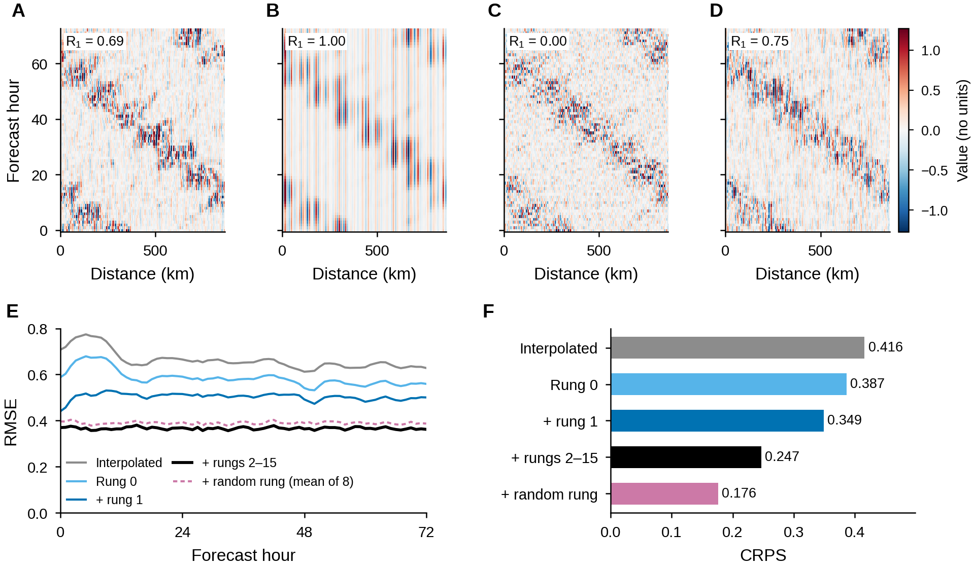
The random rung is the last rung. What the deterministic ladder (all rungs without the random one) leaves is modeled as noise and drawn at random. Its amplitude depends on the value of the estimate; its spectrum, how its variance is spread over spatial scales, and its hour-to-hour memory ρ, the fraction of each hour's noise kept in the next, are fitted on the training runs (ρ = 0.76; the texture itself was generated with 0.7, and the left-over error probably still contains a little slow error, which would raise ρ). Eight random members, an ensemble of equally likely fine fields, lower the continuous ranked probability score (CRPS) on the validation runs from 0.244 to 0.175. CRPS measures how far an ensemble is from the truth while rewarding a spread, the differences among members, that matches the actual error; lower is better, and for a single estimate it equals the mean absolute error. The score is the same whether the noise is frozen in time (0.175), redrawn every hour (0.174) or given the fitted memory, but only the fitted memory approximately reproduces how fast the texture changes. Measured on the validation runs, the correlation R1 between consecutive hours of the small scales is 1.00, 0.00 and 0.75, against 0.69 for the truth (Fig. 4, A to D). A score computed hour by hour cannot see this, although frozen or flickering detail is wrong for anything summed over hours.
One score on the test runs
On the 60 test runs the RMSE falls from 0.664 (interpolated) to 0.587 (rung 0), 0.504 (rung 1) and 0.367 (15 rungs). Each rung is lower than the one before at every one of the 73 hourly times, and after the first few hours no curve grows with forecast hour (Fig. 4E). The CRPS falls from 0.416 to 0.247 for the deterministic ladder and to 0.176 with the random rung (Fig. 4F). The mean of the eight random members has a slightly higher RMSE, 0.390, than the deterministic ladder: each member's noise has about the size of the ladder's own error, 0.367, and a mean of eight independent draws keeps one eighth of its variance, which predicts 0.367 × (9/8)1/2 = 0.389. The spread of the members, the root-mean-square difference of the members from their mean, is 0.95 times the RMSE of that mean on the validation runs; for a perfect ensemble of eight members, whose spread correctly reports how large the error is, this ratio would be (8/9)1/2 ≈ 0.94.
Discussion
The ladder is Friedman's gradient boosting (5) in which the simple model fitted at each stage has a memory. Three lessons of the original method carry over: each rung is fitted to what is still wrong, small steps keep the sequence of corrections well behaved, and the number of rungs must come from data the fit has not seen (Fig. S1 reproduces these on a curve). Two conditions are new and come from time. A rung with feedback has to be fitted the way it will be used, on its own past estimates; fitting it with the true past error gives a flattering score for a single step ahead that the model cannot reach in use. And its gain has to stay below 1, which bounds the error at every forecast hour.
The example is constructed to make each ingredient visible, and its numbers say nothing yet about real weather. The next step applies the ladder to a fine weather model run over a smaller region inside a coarse one (nested), with six variables (rain rate, surface pressure, two wind components, temperature and humidity) on two-dimensional maps. There the rungs become small neural networks that read local patches of a map and carry a state from hour to hour; the error measure can be made less sensitive to a few very large rain errors, for example the absolute error or Huber's loss, which is quadratic for small errors and linear for large ones; and the first guess can be an ensemble-conditional Gaussian process mean (1).
Materials and Methods
Test problem
The domain is periodic, 288 points of 3 km, hours 0 to 72. L is a sum of three cosine waves with wavenumbers k = 1, 2 and 3 (wavelengths across the 864-km domain), amplitudes drawn uniformly between 0.6/√k and 1.4/√k, speeds drawn uniformly between −25 and 25 km h−1, and random phases. M follows Mt = a Mt−1 + (1 − a) max(Lt, 0)2 with a = e−1/6 and M0 = max(L0, 0)2. S = (0.15 + 0.35 max(L, 0)) Z, where Z is a Gaussian random field, a set of random values along the line with a bell-shaped (normal) distribution and a prescribed spectrum, with unit variance, equal variance at wavenumbers 20 to 60 (wavelengths of 14 to 43 km) and a correlation of 0.7 between consecutive hours. The coarse input is the average of L + 0.5 max(L, 0)2 over the nine 3-km points of each 27-km cell, plus an error with a correlation of 0.9 between consecutive hours and a standard deviation of 0.1 in each cell.
Rungs
Rung 0 is the conditional Gaussian mean ŷ(0) = my + Cyu(Cuu + λI)−1(u − mu), where m are training means, C training covariances and λI a small diagonal term that keeps the inverse stable (λ is 10−3 times the mean diagonal of Cuu); the subscripts name the two variables of each covariance; this is A u + b with A = Cyu(Cuu + λI)−1. Rung 1 uses as features the interpolated coarse input at each point and at points one and two coarse cells to either side, plus a constant. Rungs 2 to 30 use 32 features max(0, qi·s + ci), with weights qi and offsets ci drawn at random once per rung and then fixed, plus a constant. Here s holds seven standardized inputs: the five interpolated coarse values, the current estimate at the point and the hourly change of the input. The weights βn come from ridge regression (penalty 10−3 times the mean diagonal of FTF, where the columns of F are the filtered features) on the filtered features; φn is chosen from {0, 0.3, 0.5, 0.7, 0.8, 0.85, 0.9, 0.95}. The recursion starts at hour 0 as if the features had been constant before. Rung 1 is added in full; rungs 2 and up are added with step size ν. Every rung is fitted out-of-fold on the five groups of training runs, so that the next rung sees errors that were not fitted. The number of rungs and ν (1 or 0.3) are those with the lowest validation RMSE.
Random rung and scores
The final out-of-fold residual r is written as σ(ŷ)w, with σ the RMS residual in 20 bins of equal population of the estimate and w a Gaussian random field with the mean spectrum of r/σ, renewed every hour as wt = ρ wt−1 + (1 − ρ2)1/2 ξt with fresh noise ξt, where ρ is the correlation of r/σ between consecutive hours. CRPS is the fair ensemble estimate, which does not favor small ensembles: the mean of |X − y| over members X, minus half the mean of |Xi − Xj| over distinct pairs of members. R1 is the correlation along the line between the field at consecutive hours after keeping only wavenumbers 17 to 144 (wavelengths shorter than 54 km).
Glossary
| rung | one successive correction; rung 0 is the first guess, rung n estimates what rungs 0 to n − 1 leave |
| random rung | the last rung; draws the unpredictable small-scale texture at random |
| deterministic ladder | all rungs without the random rung |
| feedback gain φ | fraction of a rung's previous-hour estimate carried into the next hour |
| step size ν | fraction of a rung's correction that is added |
| rollout | running a model forward hour by hour on its own estimates, as in use |
| out-of-fold | each of five groups of training runs is predicted by a fit to the other four |
| training, validation, test runs | fitting; every choice; one final score |
| RMSE, RMS, MSE | root-mean-square error; root mean square; mean squared error |
| CRPS | continuous ranked probability score: rewards accuracy and a spread matching the error; lower is better |
| ensemble, spread | several equally likely estimates; how much they differ |
| ρ, R1 | fitted hour-to-hour memory of the random rung; measured correlation of small scales between consecutive hours |
| L, M, S | waves, lagged response, small-scale texture of the test problem |
| wavenumber | number of wavelengths that fit across the 864-km domain |
| spectrum | how a field's variance is spread over spatial scales |
| filtered features | exponentially weighted averages of recent features |
| Gaussian random field | random values along the line with a normal distribution and a prescribed spectrum |
References and Notes
- S. Ravela, J. D. Kim, K. Gee, X. Yan, L. Albarghouty, A. Saha, S. Mercier, Ensemble-conditional Gaussian processes (Ens-CGP): Representation, geometry, and inference. arXiv:2602.13871 (2026).
- M. E. Levine, A. M. Stuart, A framework for machine learning of model error in dynamical systems. arXiv:2107.06658 (2021).
- M. Trautner, S. Ravela, Neural integration of continuous dynamics. arXiv:1911.10309 (2019).
- J. D. Kim, S. Ravela, R. L. Evans, The Neuro-Physical Inverter: A modular framework for magnetotelluric inversion coupling ensemble conditioning with residual learning. arXiv:2610.03225 (2026).
- J. H. Friedman, Greedy function approximation: A gradient boosting machine. Ann. Stat. 29, 1189–1232 (2001). doi:10.1214/aos/1013203451
- S. Ravela, Quantifying uncertainty for coherent structures. Procedia Comput. Sci. 9, 1187–1196 (2012). doi:10.1016/j.procs.2012.04.128
Supplementary Materials
Interactive explainer. The same method in 12 animated steps, with the numbers of this article and a glossary of every term.