
Successive correction of a generative downscaling ensemble: correct the member mean, rescale the perturbations
Research article · Estimation theory and machine learning
Successive correction of a generative downscaling ensemble: correct the member mean, rescale the perturbations
Department of Earth, Atmospheric and Planetary Sciences, Massachusetts Institute of Technology, Cambridge, MA, USA.
A generative downscaling model turns one coarse weather forecast into several equally likely fine fields for each hour, called members. A correction fitted by squared error, applied to each member, pulls every member toward the same average field and removes what makes the members differ. This article describes a chain that corrects only the mean of the members, in successive orders: a linear model with a memory of past hours (order 1), then boosting stages, each a small model of what the orders before it miss (orders 2 to N, the last order). Each member's deviation from the mean, its perturbation, is kept and only rescaled, one band of spatial scales at a time. The chain is followed box by box on a constructed one-dimensional example with 8 members per hour, whose simulated 72-hour cases (runs) are split into runs that fit the models, validation runs that choose the number of orders and the step, and test runs scored once. On 60 validation runs the root-mean-square error of the member mean falls from 0.591 to 0.427 after order 1 and to 0.363 after 18 orders, and a score of the whole ensemble (the fair continuous ranked probability score, lower is better) falls from 0.292 to 0.176; correcting each member separately with order 1 instead keeps 23% of the members' spread (how far the members differ from their mean). On 60 test runs the member-mean error is 0.370 and the score 0.178. The chain for real forecasts of six variables is being built; only the example is shown here.
A weather model run on a coarse grid misses what a finer grid resolves: rain cells, sharp fronts, winds shaped by terrain. Running the fine grid costs far more, so downscaling estimates the fine field from the coarse forecast alone. The target here is the Weather Research and Forecasting model (WRF) run on two nested grids, a coarse outer grid of 27-km cells (called d01) and a fine inner grid of 3-km cells (d03): from a 72-hour d01 forecast, the goal is the d03 fields, hour by hour, for six variables: rain rate; pressure anomaly (pressure minus the model's reference pressure); the two components of the wind 10 m above the ground; and temperature and relative humidity 2 m above the ground.
Generative models produce such fine fields as samples. CorrDiff (1) combines a regression network, which predicts the mean fine field from the coarse one, with a diffusion model, a generative network that turns random noise into a sample of the fine-scale detail around that mean. Each sample is a member, and the members of one hour form an ensemble: where they agree the estimate is confident, and where they differ (for instance in exactly where a rain cell sits) the differences express the uncertainty. The chain is built on CorrDiff μ_v2: the CorrDiff variant that starts from the Ens-CGP mean μt instead of a regression network and whose members read their own two previous hours; “v2” is its version label. The Ens-CGP mean is the mean of an Ensemble-Conditional Gaussian Process (2): the mean of the fine fields given the coarse forecast when both are treated as jointly Gaussian, with their statistics taken from a large set of training hours. The diffusion model of μ_v2 draws each member as μt plus a generated deviation; besides its own previous hours, each member also reads the coarse forecast's recent hours and the large-scale wind that steers the weather, taken from the Global Forecast System (GFS), so that its detail moves from hour to hour.
The members still have errors that a correction model could learn, such as a response that builds up hours after its cause. The obvious fix, a correction fitted by squared error and applied to every member, fails for a basic reason. A model fitted by squared error converges to the conditional mean of the truth given its inputs (the average truth over all cases with the same inputs), the single best estimate for that loss; applied to each member, it moves every member toward that same estimate, so each member loses its perturbation dk, its deviation from the mean of the members, and the ensemble collapses onto one smooth field. The chain studied here therefore corrects only the member mean, where squared error is the right loss, and gives each member back its own perturbation, rescaled by a factor α that is fitted with a score of the whole ensemble: the fair continuous ranked probability score (CRPS), the members' mean distance from the truth minus half their mean distance from one another (Materials and Methods). It is low when the members are close to the truth and differ from one another about as much as they differ from the truth. The plain ensemble CRPS penalizes small ensembles; the fair version is the estimate whose expected value equals the score of the distribution the members are drawn from, so it does not depend on the number of members.
The corrections are successive. Gradient boosting (3) builds a predictor as a sum of simple models, each fitted to what the sum so far still gets wrong, each added at a fraction ν of its size, and stops when the error on data not used for fitting stops falling. The chain uses a linear model first (order 1) and then boosting stages (orders 2 to N). Because the error of a forecast persists from one hour to the next, every correcting order (1 to N) also has a memory, a filter that carries information over from past hours. Figure 1 is the plan of the chain, box by box. The chain for real forecasts is being built; this article shows only a constructed one-dimensional example that runs every box, and its numbers say nothing yet about real weather.
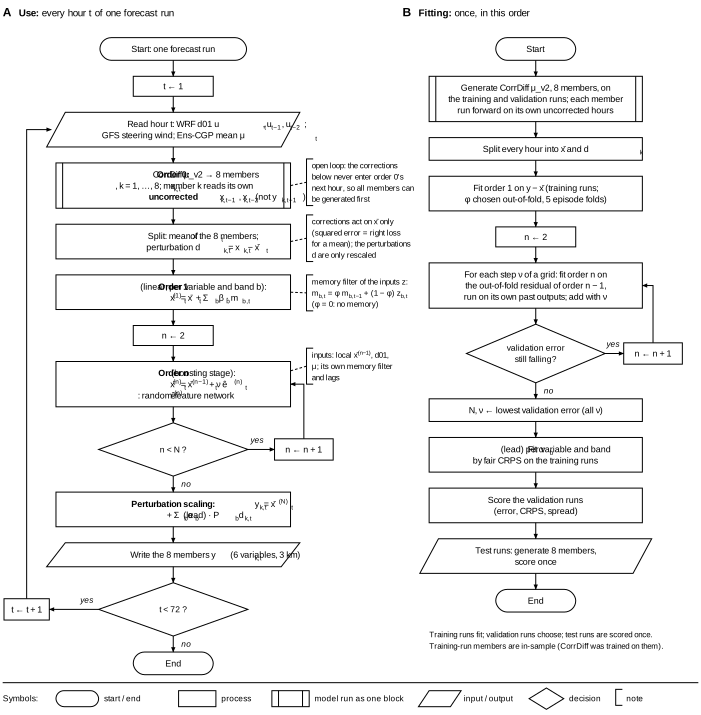
Table 1. Each box of Fig. 1 on real forecasts and in the worked example.
| box | real forecasts (being built) | worked example (shown here) |
|---|---|---|
| Start: one forecast run | a 72-hour WRF forecast | one run: 73 hourly values (hours 0 to 72) of one variable on a line |
| Read hour t | WRF d01 ut, ut−1, ut−2 (six variables, 27-km grid); GFS steering wind; Ens-CGP mean μt | one coarse series ut on 32 cells of 27 km (and ut−1 through the hourly change); no steering wind, no Ens-CGP mean |
| Order 0 | CorrDiff μ_v2: 8 members xk,t; each member reads its own two previous hours, uncorrected (open loop) | a toy generator: 8 members, each a linear map of the input plus a random part that keeps a fraction of its own previous hour's value (one hour, not two; open loop); stated defect: the random part changes faster from hour to hour than the truth's small scales |
| Split | member mean x̄t, perturbations dk,t = xk,t − x̄t | the same |
| Order 1 | linear, per variable and scale band; inputs: the current x̄, d01 and their hourly change, through a memory filter | linear, per scale band; inputs: the input at 5 points, x̄ and the hourly change of the input, through a memory filter |
| Order n | random-feature network on local x̄(n−1), the coarse forecast (d01) and μt, with its own memory filter and lags | random-feature network on local x̄(n−1), the input and its hourly change, with its own memory filter |
| Perturbation scaling | αb(lead) per variable and band | αb(lead) per band (one variable) |
| Write the members | 8 members, six variables, 3 km | 8 members, one variable, 3-km points |
| Fitting: runs and folds | training, validation and test runs; 5 folds of whole weather episodes | 240 training, 60 validation and 60 test runs; 5 folds of runs (run number modulo 5) |
Results: using the chain, every hour t of one forecast run (Fig. 1A)
The worked example
The example is a constructed test problem with a known truth. A periodic line of 864 km (its right end joins its left end) is seen by a coarse model in 32 cells of 27 km and by a fine model at 288 points 3 km apart, hourly from hour 0 to hour 72. One run is one such realization. The values have no units. The fine truth y (written without a member index; yk,t with an index is an output member, an estimate of it) is, by design, the sum of three parts, y = L + M + S (Table 2 and fig. S1). Each part stands for one kind of predictability and so tests one part of the chain: L can be predicted from the same hour of the coarse input, M mostly from its past, and S not at all, only its statistics. On real forecasts the truth (the d03 field) is not split into such parts; in Fig. 1 the truth appears only in panel B, where the orders are fitted to it (“Fit order 1 on y − x̄”).
Table 2. The three parts of the example's truth y = L + M + S. t is the hour; the forcing g = max(L, 0)2 is the positive part of L, squared. Formulas in Materials and Methods.
| part | what it is | predictable from | boxes of Fig. 1 it tests |
|---|---|---|---|
| L | large travelling waves: 3 waves with wavelengths of 288 to 864 km, each with a random speed between −25 and 25 km h−1 | the same hour of the input | Read hour t; Order 0 (a map from the same hour) |
| M | a lagged response to the forcing g, that is to L where L is positive: Mt = a Mt−1 + (1 − a) gt with a = e−1/6 ≈ 0.85, an average of past forcing that forgets on a 6-hour time scale, so M peaks hours after g | mostly the past of the input (the current hour's forcing enters with weight 1 − a ≈ 0.15) | the memory filters of Order 1 and Order n (on real forecasts also their lags); the square, a nonlinearity, is for the boosting stages of Order n |
| S | a small-scale part with wavelengths of 14 to 43 km, too short for the coarse cells (a grid needs at least two cells per wavelength, 54 km here); each hour it keeps a fraction 0.7 of its previous pattern and adds new random detail; its size is 0.15 + 0.35 max(L, 0) | its size, from L; its pattern, from nothing | Split (the members' perturbations dk); Perturbation scaling |
The coarse input u is the average over each 27-km cell of L + 0.5g, plus an error of its own that changes slowly from hour to hour. It therefore sees the forcing g at once and at half strength, not the lagged full response M, and none of S. There are 360 runs: 240 training runs fit every model, 60 validation runs choose the number of orders and the step (the other constants are fitted on the training runs), and 60 test runs are scored once, at the end. Errors are root-mean-square errors (RMSE): the square root of the mean squared difference from the truth over all points, hours and runs (over one run when a figure prints it). Every figure shows the same run, the first validation run, and its 1-D panels show the field along the line at hour 36, marked by triangles on the Hovmöller diagrams, maps of the field with position along the line across and the hour upward; a feature that travels along the line appears there as a slanted stripe. The hour-to-hour correlation of a pattern, used below, is the correlation along the line between the field at one hour and at the next, averaged over hours and runs: 1 means the pattern does not change. Each figure of a box shows that box's input (the field the box receives), its change (output minus input), its output, the truth, and the error before and after the box (estimate minus truth), all on the same two color scales in every figure. A residual is the opposite, truth minus estimate: what a correction has to add.
Start: one forecast runstart / end
The chain starts from one coarse forecast run, hours 1 to 72 on real forecasts. The example's runs also have the initial hour 0, so they have 73 hourly values, and the chain processes all of them.
t ← 1process
The hour counter starts at the first hour, t = 1 on real forecasts and t = 0 in the example, where the loop runs over hours 0 to 72. The memory filter of each correcting order starts from that first hour: before it there is no past, so the filter's state is set to the first hour's inputs.
Read hour tinput / output
The chain reads the coarse input of hour t and of the hours before it. In the example that is the coarse value ut of each 27-km cell; the boxes below use it as interpolated linearly between the centers of the cells to the 3-km points (Fig. 2). The interpolated input already follows the large waves L, but it misses the lagged response M, which peaks after the input does, and the small-scale part S: its validation RMSE is 0.621.

Order 0: CorrDiff μ_v2 → 8 membersmodel run as one block
On real forecasts order 0 is CorrDiff μ_v2. In the example it is a toy generator fitted on the training runs: each member is xk = A u + q + ηk, k = 1, …, 8. The mean part A u + q is the least-squares linear map of the coarse input of the same hour (validation RMSE 0.556); the random part ηk, different for every member, has the spatial structure and the hour-to-hour correlation of what that map misses on the training runs. The toy generator is given one defect on purpose: its random part gets a weaker hour-to-hour correlation than it was fitted with, so its fine detail changes faster from hour to hour than the truth's. At wavelengths below 30 km, where S mostly lies, the hour-to-hour correlation of the members' pattern on the validation runs is 0.59, against 0.69 for the truth (Table 3). A single member carries detail everywhere, which makes its RMSE (0.797) larger than that of the smooth interpolated input (Fig. 3): a member is one equally likely sample, and the best single estimate is their mean (next box).
Order 0 runs open loop: a member's next hour is built from its own uncorrected previous hours, never from the corrected output yk,t. The corrections of the boxes below therefore never enter order 0's step from one hour to the next: the members carried forward are order 0's own, and each correcting order carries forward only its own memory filter and lags. That is why all members of all hours can be generated first (panel B) and the orders fitted afterwards. Feeding the corrected output back (closed loop) would keep errors already removed by the orders out of the next hour. It is not used because the generator learned from its own outputs, so corrected inputs would be unlike its training inputs, and because every fitted order would require generating the members again.

Table 3. Hour-to-hour correlation of the pattern, per scale band. The correlation along the line between a band's field at one hour and at the next, averaged over hours and runs (1: the pattern does not change). The toy generator's random part is given a weaker correlation on purpose. Below 30 km, where the members are almost all perturbation, the scaling leaves the correlation as order 0 made it; in the larger bands the output members come closer to the truth's correlation, because their mean part is now the corrected mean and α < 1 shrinks the perturbations there.
| band | truth, validation | order-0 members, validation | output members, validation | truth, test | output members, test |
|---|---|---|---|---|---|
| above 300 km | 0.99 | 0.98 | 0.99 | 0.99 | 0.99 |
| 30 to 300 km | 0.93 | 0.89 | 0.92 | 0.94 | 0.93 |
| below 30 km | 0.69 | 0.59 | 0.59 | 0.69 | 0.59 |
Split: member mean and perturbationprocess
The members of hour t are split into their mean x̄t = (1/8) Σk xk,t and the perturbations dk,t = xk,t − x̄t, each member's deviation from the mean (Fig. 4). Averaging removes most of the detail that differs between members, so the mean is closer to the truth than any one member: validation RMSE 0.591 for x̄ against 0.797 for member 1. The random parts of 8 members do not cancel completely: their mean keeps 1/8 of their variance. From here on the corrections act on x̄ only; the perturbations are kept unchanged until the perturbation scaling box.

Order 1 (linear, per variable and band b)process
Order 1 is a linear model of the residual of the member mean, y − x̄. It works separately in three bands of spatial scales: Pb keeps the scales of band b of a field, wavelengths above 300 km, 30 to 300 km, and below 30 km, and the three parts add up to the field. Its inputs in band b, zb,t, are band b of the coarse input at the point and at one and two cells to either side, of the current x̄t, and of the hourly change of the input (Materials and Methods). The inputs pass through a memory filter, mb,t = φ mb,t−1 + (1 − φ) zb,t, an average over past hours in which an hour h hours ago counts with weight proportional to φh; φ = 0 means no memory, and with φ < 1 an error made at one hour fades instead of growing. The corrected mean is
x̄(1)t = x̄t + Σb βb · mb,t,
with weights βb and the constant φ of each band fitted in panel B (Table 4). It lowers the validation RMSE of the member mean from 0.591 to 0.427; without memory (φ = 0 in every band) it reaches only 0.471. In Fig. 5 its correction removes part of the slanted stripes of the lagged response M.

n ← 2process
The loop over boosting stages starts at order 2, the first order after the linear one.
Order n (boosting stage)process
Order 1 is linear, but the lagged response is not: it follows the square of the waves. Each boosting stage n adds a nonlinear model of the residual of orders 1 to n − 1,
x̄(n)t = x̄(n−1)t + ν ê(n)t,
where the correction ê(n)t comes from a random-feature network: 32 hidden units, each the positive part, max(0, ·), of a weighted sum of 7 local inputs (the input at 5 points, x̄(n−1)t and the hourly change of the input), with weights drawn at random once and then fixed; only the output weights are fitted, by ridge regression (least squares with a small penalty on the size of the weights), on the hidden units' outputs passed through the stage's own memory filter. Each correction is added at the step ν, the fraction of it that is added. The stage reads its own past outputs through that filter, never the true past error, which is not known when the chain is used. The first stage lowers the validation RMSE of the member mean from 0.427 to 0.382; all stages up to N = 18, each added in full (ν = 1), lower it to 0.363 (Fig. 6). The broad slanted stripes of the lagged response M are gone; what remains are the fine streaks of the small-scale part S.

n < N ?decision
If n < N, the counter moves to n + 1 and the next stage corrects the output of this one. N = 18 and ν = 1 were chosen on the validation runs (panel B, Table 5). Movie 1 runs this loop for the example: M's stripes fade over the first stages, S's streaks stay, and later stages change the error little.
Perturbation scalingprocess
Each member gets its own perturbation back, rescaled band by band:
yk,t = x̄(N)t + Σb αb(lead) · Pb dk,t,
where lead is the forecast hour t and αb(lead) is one factor per band and hour, fitted in panel B (Table 6). The perturbations of the 8 members sum to zero, so the mean of the output members is x̄(N) itself; the scaling sets only how far the members spread around it. Each output member, a sample, has a larger RMSE than the corrected mean (0.522 for member 1 against 0.363; Fig. 7), but the ensemble as a whole scores better than the corrected mean alone (Table 7). The perturbations keep order 0's defect (Table 3): rescaling changes the size of a perturbation and leaves its hour-to-hour behavior as it was.

Write the 8 membersinput / output
The 8 members yk,t of hour t are written out. Figure 8 compares what is written with what order 0 produced: each member keeps its own detail, while the member mean, now x̄(N), has lost most of the lagged response's error (validation RMSE of the member mean 0.591 for order 0, 0.363 written).

t < 72 ?decision
If t < 72, the counter moves to t + 1 and the chain reads the next hour. The memory filters keep their state from hour to hour; together with the lags and order 0's own uncorrected previous hours (open loop), they carry information from hour t − 1 to hour t. Movie 2 runs this loop for the example, hour by hour, through the main boxes.
Endstart / end
The run's output is complete: 8 members for each of its hours.
Fitting: once, in this order (Fig. 1B)
All parts are fitted once, before the chain is used, in the order in which they run.
Startstart / end
Fitting needs the coarse input and the truth of every run in the three sets.
Generate CorrDiff μ_v2, 8 members, on the training and validation runs, each member run forward on its own uncorrected hoursmodel run as one block
Order 0 is run on every training and validation run, each member run forward hour by hour on its own uncorrected previous hours (open loop, so this can be done once, before any order is fitted): on real forecasts the already trained CorrDiff μ_v2, in the example the toy generator. (For convenience the example also generates the test-run members here, from their input only; the chart generates them in its last box, where they are first needed.) CorrDiff μ_v2 was trained on the training runs, so its members there are in-sample, produced by a model fitted on those same runs, and closer to the truth than on new runs. The example's generator is likewise fitted on all training runs. Corrections fitted on in-sample members may come out too small. The chain is nevertheless fitted on the in-sample members, as it will be on real forecasts, where the generator is used as trained. To measure the effect, the toy generator was refitted 5 times, each time without one group of training runs, which gives out-of-fold members, and order 1 was fitted once on each kind (Fig. 9). On the same training runs the RMSE of the member mean is 0.5970 in-sample against 0.6043 out-of-fold; on the validation runs the correction of the in-sample fit is 1.3% smaller in RMS (root-mean-square) size overall and 5.5% smaller below 30 km, and the validation RMSE after order 1 is 0.4273 against 0.4271. The effect is small here because the toy generator has few fitted coefficients; a neural network with many more fitted parameters may fit its training runs more closely, and then the effect on real forecasts would be larger; the validation runs will show it.

Split every hour into x̄ and dkprocess
As in use, every hour of every run is split into the member mean and the perturbations.
Fit order 1 on y − x̄process
Order 1 is fitted to the residual of the member mean, y − x̄, on the training runs, not to the residual of each member. Figure 10 shows why. Fitted by squared error to the residual of every member, y − xk, with the member itself among its inputs, the same model learns to remove the member: its weight on the member is between −1.03 and −0.99 in every band, so each corrected member is rebuilt from the coarse input alone. The alternative is order 1 fitted to the residual of the mean, with the perturbations rescaled afterwards by an α fitted as in panel B (the chain without boosting stages). Over all validation runs, correcting each member keeps 23% of the members' spread, the typical difference of the members from their mean (Materials and Methods), against 82% for correcting the mean, and its fair CRPS is worse, 0.267 against 0.213. Member 1's RMSE is lower after correcting each member, 0.462 against 0.607 after correcting the mean; this reflects the collapse, since a member without its perturbation lies close to the mean. Figure 10 prints the values of its one run, which are close to these (member 1's RMSE after correcting each member rounds to 0.462 on that run too). Fitted to the mean, order 1 also gives x̄ a strongly negative weight (−0.80 to −0.94, Table 4): it partly replaces the member mean by its own estimate from the input and its memory. For the mean this is harmless, because the perturbations are added back afterwards; applied to each member, a weight near −1 removes the member's own detail.
The constant φ of each band is chosen from {0, 0.3, 0.5, 0.7, 0.8, 0.85, 0.9, 0.95} by out-of-fold error: the training runs form 5 groups, each group is predicted by weights fitted on the other groups, and the φ with the lowest error on these predictions is kept (Table 4). Every training run's correction is computed the same way, out-of-fold, so that the next order learns from errors that were not fitted already: an in-sample correction would make the residual on the training runs look smaller than it is on new runs. Memory helps at large scales (φ = 0.8 and 0.85); below 30 km the out-of-fold error is lowest without it (φ = 0).

Table 4. Order 1 per scale band. φ chosen out-of-fold on the training runs; validation RMSE of the band's part of the member mean before (x̄) and after order 1 (x̄(1)); the weight on x̄ shows that order 1 damps the member mean and rebuilds the field from the input and its memory.
| band | φ | weight on x̄ | RMSE x̄ | RMSE x̄(1) |
|---|---|---|---|---|
| above 300 km | 0.8 | −0.80 | 0.369 | 0.182 |
| 30 to 300 km | 0.85 | −0.89 | 0.326 | 0.234 |
| below 30 km | 0 | −0.94 | 0.328 | 0.308 |
n ← 2process
The stages are fitted one after another, starting with order 2, each on what the orders before it miss.
For each step ν of a grid: fit order n on the out-of-fold residual of order n − 1process
Stage n is fitted on the training runs to the residual y − x̄(n−1), where x̄(n−1) is out-of-fold. Its random input weights are drawn once; its output weights and its φ are fitted as for order 1, with the stage run on its own past outputs, exactly as in use. It is then added with step ν. The grid of steps here has two values, ν = 1 (each correction added in full) and ν = 0.3; for each, up to 30 orders were fitted.
Validation error still falling?decision
After each stage the validation RMSE of the member mean is computed. The chart stops at the first rise; the example instead fits all 30 orders for each step and keeps the lowest, which also shows what happens after it (Table 5). With ν = 1 the validation error falls until order 18 and then rises, and the size of each stage's correction shrinks only until order 10 and then grows. The out-of-fold training error, the RMSE of the out-of-fold corrected mean on the training runs, is lowest at order 8 (0.3728) and then rises, to 0.4897 at order 30, far above the validation RMSE there (0.3906). A likely reason: out-of-fold corrections keep the training residual as large as it would be on new runs, but they come from 5 fits, one per fold, that differ slightly. On the training runs the residual that the next stage sees therefore contains, besides the real error, the differences between these fits; the stage learns part of them and adds them back, and with full steps the following stages repeat this, so the training error grows. On the validation runs every correction comes from the one fit on all training runs, so these differences do not arise there. The effect is largest above 300 km, where the corrections are large (order 1 alone lowers that band's validation RMSE from 0.369 to 0.182, Table 4) and the error left at the end is small (0.067), so slight differences between the fold fits are large compared with it. With ν = 0.3 each stage adds only part of its correction: the corrections shrink by about a factor of ten from order 2 to order 30, with their smallest at order 25, the validation error is still falling slowly at order 30, and the out-of-fold training error stays close to it (0.3755 against 0.3677 at order 30). Within 30 orders the small step behaves much better, although 30 orders cannot show that it converges.
N, ν ← lowest validation error (all ν)process
The lowest validation RMSE over both steps is kept: ν = 1 with N = 18 (0.4273 after order 1, 0.3635 after order 18). The small step at N = 30 is within 1.2% of it.
Table 5. Choosing N and ν on the validation runs. RMSE of the member mean; “out-of-fold training” is the error of the out-of-fold corrections on the training runs; correction size is the RMS of a stage's added correction, νê(n), on the validation runs.
| step ν | lowest validation RMSE (at order) | validation RMSE at order 30 | lowest out-of-fold training RMSE (at order) | correction size, order 2 → 30 | smallest correction at order |
|---|---|---|---|---|---|
| 1 | 0.3635 (18) | 0.3906 | 0.3728 (8) | 0.1827 → 0.1034 | 10 |
| 0.3 | 0.3677 (30) | 0.3677 | 0.3747 (22) | 0.0548 → 0.0056 | 25 |
Fit αb(lead) per variable and band by fair CRPS on the training runsprocess
For each band and each forecast hour, αb minimizes the fair CRPS of the band's part of the members, Pb x̄(N) + αb Pb dk, against the band's part of the truth on the training runs, with the out-of-fold x̄(N). Each band is scored on its own, because the score of the whole field fixes only the total spread at each point, not how it divides among the bands. Within one band the score is convex in α, so it has a single minimum, and the fitted factors change smoothly with the hour (Table 6). α shrinks the large-scale perturbations most; below 30 km it stays near 1, because order 0's fine detail already has about the right size there and no order can predict it.
The spread-to-error ratio checks the result: the members' spread divided by the RMSE of their mean. For these members, the corrected mean plus perturbations centered on it, a ratio of 1 means the spread matches the error (for order 0's members, which are averaged into their own mean, the ideal is 0.94 instead; Materials and Methods). On the training runs, where α was fitted, the ratio is 1.02, close to 1 although a fair-CRPS fit can lean higher (for a Gaussian error the fair CRPS is lowest at a ratio of 1.23; Materials and Methods). On the validation runs it is 1.10 overall but 2.54 above 300 km. The reason is the rise of the out-of-fold training error described above: α is fitted on the training runs so that the members' spread matches the error of the out-of-fold x̄(N) there, and above 300 km that training error (0.142) is about twice the validation error (0.067). The members' spread is about the same on both sets of runs, so the training ratio in that band, 1.19, becomes about 1.19 × 0.142/0.067 ≈ 2.5 on the validation runs.
Table 6. Perturbation scale αb(lead) per band. Mean, minimum and maximum over the 73 hours; mean change from one hour to the next; spread-to-error ratio of the output members on the training runs (where α was fitted) and on the validation runs.
| band | α mean | α range | hourly change | spread/error, training | spread/error, validation |
|---|---|---|---|---|---|
| above 300 km | 0.47 | 0.35–0.49 | 0.0063 | 1.19 | 2.54 |
| 30 to 300 km | 0.69 | 0.65–0.72 | 0.0062 | 1.09 | 1.16 |
| below 30 km | 0.96 | 0.94–0.97 | 0.0056 | 0.95 | 0.97 |
Score the validation runs (error, CRPS, spread)process
With every part fixed, the chain is scored on the validation runs (Table 7), with the three scores named in the box: the error (RMSE), the fair CRPS and the spread (as the spread-to-error ratio). The RMSE of the member mean falls from order 0 to order 1 to order 18. The output members have the lowest fair CRPS: 0.176, against 0.292 for the order-0 members, 0.248 for the corrected mean used alone as a single estimate, and 0.185 for the corrected mean plus the unscaled perturbations (α = 1).
Test runs: generate 8 members, score onceinput / output
The test runs are read once, after everything else is fixed; no choice depends on them. They repeat the validation results (Table 7): the RMSE of the member mean falls from 0.619 (order 0) to 0.439 (order 1) and 0.370 (order 18), the fair CRPS from 0.302 to 0.178, and the band above 300 km again has too much spread (spread-to-error ratio 2.46). The hour-to-hour correlations repeat those of the validation runs (Table 3).
Table 7. Scores on the validation runs and, once, on the test runs. RMSE of one member or of the member mean; fair CRPS of the members (of a single estimate, its mean absolute error); spread-to-error ratio of the members.
| after box | field | validation | test |
|---|---|---|---|
| Read hour t | RMSE, input on the 3-km points | 0.621 | 0.664 |
| Order 0 | RMSE, member 1 | 0.797 | 0.804 |
| Split | RMSE, member mean x̄ | 0.591 | 0.619 |
| Order 1 | RMSE, x̄(1) | 0.427 | 0.439 |
| Order N = 18 | RMSE, x̄(N) | 0.363 | 0.370 |
| Perturbation scaling | RMSE, member 1 | 0.522 | 0.526 |
| Read hour t | fair CRPS, input alone | 0.399 | 0.416 |
| Order 0 | fair CRPS, members | 0.292 | 0.302 |
| Order N = 18 | fair CRPS, x̄(N) alone | 0.248 | 0.250 |
| Perturbation scaling | fair CRPS, output members | 0.176 | 0.178 |
| Order 0 | spread/error, members | 0.96 | 0.91 |
| Perturbation scaling | spread/error, output members | 1.10 | 1.08 |
| Perturbation scaling | spread/error, above 300 km | 2.54 | 2.46 |
Endstart / end
The example runs every box of Fig. 1 and supports the design: correct the mean, keep the perturbations, choose N and ν on runs not used for fitting. It also shows three things to watch on real forecasts. The in-sample effect of order 0's training runs can be larger for a neural network than for the toy generator. α inherits any gap between the out-of-fold training error and the validation error, band by band, as above 300 km here. And the scaling sets the size of the perturbations but leaves their behavior in time as order 0 made it: order 0's defect reaches the written members.
Materials and Methods
The example's truth and input
The line has 288 points 3 km apart (period 864 km); a coarse cell is the average of 9 points. At position s and hour t, L(s, t) = Σj=13 κj cos(2πj(s − cj t)/864 km + θj), with amplitude κj uniform between 0.6/√j and 1.4/√j, speed cj uniform between −25 and 25 km h−1 and phase θj uniform. With g = max(L, 0)2, Mt = a Mt−1 + (1 − a) gt, a = e−1/6, M0 = g0. S = (0.15 + 0.35 max(L, 0)) ζ, where ζ is a Gaussian random field (random values along the line with a normal distribution and a prescribed distribution of variance over wavelengths) with unit variance and equal power at wavenumbers (wavelengths per period) 20 to 60, renewed as ζt = 0.7 ζt−1 + (1 − 0.72)1/2 ξt with fresh random fields ξt. The coarse input is u = cell average of (L + 0.5 g) + ε, where the cell error ε has standard deviation 0.1 and keeps a fraction 0.9 of itself from one hour to the next. The bands are: above 300 km, wavenumbers 0 to 2; 30 to 300 km, 3 to 28; below 30 km, 29 to 144; Pb keeps the Fourier coefficients of band b, the amplitudes of the cosine and sine waves that make up the field.
Order 0
A = Cyu(Cuu + λI)−1 and q = ⟨y⟩ − A⟨u⟩, from the training-run means ⟨·⟩ and covariances C of the fine truth and the coarse input (A maps the 32 cell values of u to the 288 points; I is the identity matrix), with λ = 10−3 times the mean variance of the input. The random part ηk has, at each wavenumber, the power of the training residual y − (A u + q) and evolves in time as a first-order autoregressive process (each hour keeps a fraction ρ of the previous hour's value and adds fresh noise); ρ is the residual's hour-to-hour correlation at that wavenumber, multiplied by a factor below 1 in each band (the stated defect), smallest at the finest scales. The same random numbers are used for every refit.
Order 1 and the boosting stages
Order 1's inputs at each point are the coarse input interpolated to the point and to the points one and two cells to either side (5 values), the field being corrected, the hourly change of the interpolated input (zero at the first hour) and a constant (in the largest-scale band only), each projected on band b. A stage's inputs are 7 local values, standardized to zero mean and unit variance (the 5 input values, x̄(n−1) and the hourly change of the input); with r the vector of these inputs, its 32 hidden units are max(0, wi·r + oi) with weight vectors wi and offsets oi drawn once from a normal distribution, plus a constant. In both, with zt the inputs (order 1) or the hidden units' outputs (a stage) at hour t, the correction is êt = β·mt with mt = φmt−1 + (1 − φ)zt and m0 = z0. This equals the recursion êt = φêt−1 + (1 − φ)β·zt run on its own outputs, so for a fixed φ the fit is a ridge regression on the filtered inputs (penalty 10−3 times the mean, over inputs, of the sum of squares of a filtered input); φ is chosen from {0, 0.3, 0.5, 0.7, 0.8, 0.85, 0.9, 0.95} by out-of-fold error over 5 groups of runs (run number modulo 5).
Scores
RMSE is the root of the mean squared difference from the truth over all points, hours and runs. The fair CRPS of K members x1, …, xK against the truth y at one point is (1/K) Σk |xk − y| − Σi<j |xi − xj| / (K(K − 1)), averaged over points, hours and runs; the first term rewards members close to the truth, the second rewards spread. Dividing the pair sum by K(K − 1) rather than K2 makes its expected value the score of the distribution the members are drawn from, whatever the number of members; the plain ensemble CRPS, with K2, penalizes small ensembles. For one estimate (K = 1) only the first term is kept: the mean absolute error. The spread is the square root of the mean, over points, hours and runs, of the members' variance about their mean, with the sum of squares divided by K − 1; the spread-to-error ratio divides it by the RMSE of the member mean. For the order-0 members, independent draws averaged into their mean, the ideal ratio is (K/(K + 1))1/2 = 0.94 (validation: 0.96); for the output members, the corrected mean plus perturbations centered on it, it is 1. A fair-CRPS fit of α can lean above 1. With the truth at a Gaussian distance δ ~ N(0, 1) from the corrected mean and members at σ(ωk − ω̄) from it, ωk ~ N(0, 1) independent with mean ω̄, the expected fair CRPS is (2/π)1/2[((K − 1)σ2/K + 1)1/2 − σ/21/2], since xk − y and xi − xj are Gaussian with variances (K − 1)σ2/K + 1 and 2σ2. It is smallest at σ = K/[(K − 1)(K − 2)]1/2, and σ is the spread-to-error ratio: 1.23 for K = 8. The hour-to-hour correlation of a pattern is the correlation along the line between a band's field at consecutive hours, averaged over hours and runs.
Glossary
| downscaling | estimating a fine-grid field from a coarse-grid forecast |
| WRF, d01, d03 | Weather Research and Forecasting model; its coarse outer grid (27 km) and fine inner grid (3 km) |
| GFS, steering wind | Global Forecast System; the large-scale wind that moves weather systems along |
| member, ensemble | one equally likely sample of the fine field; the set of members of one hour |
| CorrDiff, CorrDiff μ_v2 | a generative downscaling model: a regression network for the mean plus a diffusion model for the detail (1); the CorrDiff variant used here, which starts from the Ens-CGP mean μt instead of a regression network and whose members read their own two previous hours (“v2” is its version label) |
| Ens-CGP mean μt | mean of an Ensemble-Conditional Gaussian Process: the fine fields' mean given the coarse forecast, both treated as jointly Gaussian, statistics from a large set of training hours (2) |
| ut, y | coarse input at hour t; fine truth (no member index) |
| error, residual | estimate minus truth; truth minus estimate, what a correction has to add |
| L, M, S, g | the example's truth y = L + M + S: large travelling waves; lagged response to the forcing g = max(L, 0)2; small-scale part |
| xk,t, x̄t, dk,t | order-0 member k at hour t; mean of the members; perturbation xk,t − x̄t |
| order n, x̄(n)t | level n of the successive correction (0: generator, 1: linear model, 2 to N: boosting stages); the member mean after order n |
| open loop, closed loop | open loop: order 0 builds each member's next hour from its own uncorrected previous hours, never from the corrected output, so the corrections do not enter order 0's step in time (used here); closed loop: the corrected output would be fed back instead |
| boosting stage, ê(n)t, ν, N | one order from 2 on, a model of the residual left by the orders before it; its correction; the fraction of it added; the last order |
| random-feature network | a network with one layer of hidden units whose input weights are drawn at random and fixed; only its output weights are fitted |
| ridge regression | least squares with a small penalty on the size of the weights |
| memory filter mt, memory constant φ | mt = φmt−1 + (1 − φ)zt, an average over past hours; φ < 1, so a past error fades as φh after h hours |
| zb,t, βb | inputs of order 1 in band b; their fitted weights |
| scale band, Pb, wavenumber | a range of wavelengths (above 300, 30 to 300, below 30 km); keeps that range of a field; number of wavelengths per period of the line |
| αb(lead), lead | perturbation scale for band b; the forecast hour t |
| yk,t | output member k at hour t |
| training, validation, test runs | runs that fit the models; runs that choose the number of orders and the step; runs scored once at the end |
| fold, out-of-fold, in-sample, out-of-fold training error | one of the groups the training runs are split into; predicted by a fit that did not use the run's fold; predicted by a fit that used the run itself; RMSE of the out-of-fold corrected mean on the training runs |
| RMSE, RMS | root-mean-square error; root mean square |
| fair CRPS | fair continuous ranked probability score of an ensemble; lower is better (Materials and Methods) |
| spread, spread-to-error ratio | how far the members differ from their mean; spread divided by the RMSE of the member mean |
| Hovmöller diagram | a map of a field with position across and time upward |
| hour-to-hour correlation | correlation along the line between a field at one hour and at the next; 1: the pattern does not change |
References and Notes
- M. Mardani, N. Brenowitz, Y. Cohen, J. Pathak, C. Y. Chen, C. C. Liu, A. Vahdat, K. Kashinath, J. Kautz, M. Pritchard, Generative residual diffusion modeling for km-scale atmospheric downscaling. arXiv:2309.15214 (2023).
- S. Ravela, J. D. Kim, K. Gee, X. Yan, S. Mercier, L. Albarghouty, A. Saha, Ensemble-conditional Gaussian processes (Ens-CGP): Representation, geometry, and inference. arXiv:2602.13871 (2026).
- J. H. Friedman, Greedy function approximation: A gradient boosting machine. Ann. Stat. 29, 1189–1232 (2001). doi:10.1214/aos/1013203451
Supplementary Materials
